Book map: measure, clean, represent, infer, fuse, deploy

"They gave me six verbs and swore the whole book was hiding inside them. It was annoying how completely correct that turned out to be."

A Well-Read AI Agent

Virtually every sensory-AI system ever shipped runs on the same six-word sentence, whether a two-dollar fall detector or a full self-driving stack. The rest of this book is the dictionary for it. Section 1.5 walked one signal through that sentence at the scale of a single sensing chain, from raw transduction to a decision. This section zooms all the way out and applies the same idea at the scale of the whole volume. The prerequisite is light: you need only the shared vocabulary built earlier in this chapter, the four quantities from Section 1.3 (a signal \(x(t)\) or \(x[n]\), a hidden state \(s\), an event \(e\), an action \(a\)), the measurement model \(x = h(s) + \eta\), and a learned representation \(z\). Those symbols are the alphabet; the six verbs are the grammar that arranges them into a working system. The full symbol table lives in Appendix J, Notation and Glossary, and the concrete route-planning advice lives in Front Matter F4, How to Use This Book; this section is the bridge between them.

The six-verb arc as the spine of the book

When a self-driving car brakes for a phantom obstacle or a wrist wearable misses a real arrhythmia, the hardest question on the team is often not how to fix the bug but where the error entered in the first place. The six-verb arc exists to answer exactly that, and to answer it before you write a single line of debugging code. What the arc is: an ordered sentence that every sensory-AI system speaks. You measure to obtain \(x\) from the world through an imperfect sensor \(h(\cdot)\). You clean to suppress the noise \(\eta\) and produce a conditioned observation \(y\). You represent to compress \(y\) into a feature or embedding \(z\) (a learned vector that places inputs with similar structure near each other) that exposes the structure a decision needs. You infer to estimate the hidden state \(\hat{s}\), or an event \(e\), from \(z\). You fuse to combine several sensors or several times into one coherent estimate. You deploy to run all of it reliably under the power, latency, and privacy budgets of Section 1.6. Why six and not one end-to-end box: even a model trained end-to-end still performs these functions internally, and naming them separately is what lets you reason about where an error entered, which stage to fix, and which chapter teaches the fix.

How the arc maps onto the fourteen Parts is the actual map, drawn in Figure 1. The mapping is many-to-many on purpose: infer is the widest verb because most of the book is inference under a different sensor, while clean is narrow because classical signal conditioning concentrates in one Part. When to consult it: any time you feel lost, ask which verb the current chapter serves, and the arc tells you what came before it and what it feeds. In short: name the verb a chapter serves and you instantly know what feeds it, what it feeds, and where to look when the output is wrong.

Reading only your level: the [F], [C], [A], [R] tags

The verbs place a chapter on the arc, but they say nothing about how deep it dives, and that second dimension is exactly what the level tags supply. Three audiences share this one book, and the level tags are how they avoid reading each other's chapters. What the tags mean: [F] foundational, the shared floor everyone needs; [C] core, the working methods a practitioner uses daily; [A] advanced, the harder machinery for specialists; [R] research frontier, the 2023 to 2026 techniques that are still moving. Every chapter carries a tag in its header, and many carry two (Chapter 5 is [F][C], Chapter 16 is [A][R]) to signal that they straddle a boundary. Why this matters: an advanced undergraduate can read every [F] and most [C] chapters and come away with a complete, honest picture, while safely skimming the [R] material. A practicing engineer can go straight to the [C] and [A] chapters for their modality and treat the [F] chapters as a reference to dip into. How to use them with the verbs: pick your verbs (your job), then pick your level (your depth), and the intersection is your reading path.

Those paths are named explicitly in Front Matter F4: an undergraduate track that stays in the [F] and [C] spine, a graduate track that adds the [A] and [R] chapters, and role tracks for edge, robotics, health, and industrial readers that select the Parts matching a deployment domain. The edge track, for instance, threads from deploy in Chapter 59, Edge AI Fundamentals and Model Optimization back through whichever infer chapter serves its modality, rather than reading the volume in Part order.

Five running threads that recur all the way to the capstone

Verbs and levels together pin down where a chapter sits and how deep it goes, yet a third kind of structure runs sideways through every one of them. Some ideas are too important to confine to one chapter, so the book weaves them as recurring threads. What the five threads are: leakage-safe evaluation (never let information from the test window inform training), uncertainty and calibration (a \(\hat{s}\) without a trustworthy confidence is half an answer), sensor failure modes (drift, saturation, dropout, and spoofing are the rule, not the exception), biometric and privacy ethics (a heartbeat or a gait is an identity), and the classical-versus-foundation-model tradeoff (when a Kalman filter (the classical recursive state estimator) beats a transformer, and when it does not). Why thread them rather than chapter them: each one applies to every verb, so pinning it to a single location would falsely imply it is done once and forgotten. How they resurface: a leakage-safe split appears the moment any model is trained, in Part IV as much as in Part VIII; calibration appears wherever a decision rides on a probability. When they converge: all five reunite in Chapter 72, Frontier Research and the End-to-End Capstone, where you build one system that measures, cleans, represents, infers, fuses, and deploys, and every thread is graded at once.

The most easily botched of the five is leakage-safe evaluation, because the mistake is invisible: a model that peeked at the future reports a beautiful score and then fails in the field. The discipline is developed in full in Chapter 5, Sensor Data Engineering and Leakage-Safe Datasets, and the single most common fix, grouping by subject or session so no person straddles the train and test sets, is a one-liner with the right tool.

Precisely, leakage is any path by which information tied to a test sample reaches the model during training. Leakage-safe evaluation is a splitting rule that closes those paths, so the reported score estimates true unseen-data performance. It matters because leakage silently inflates accuracy: the model memorizes a shortcut (this subject's resting heart rate, this session's sensor bias) instead of the target relationship, and the inflated number collapses in deployment. The fix defines a grouping key, such as subject, session, or a time boundary, and forces every correlated sample onto one side of the split so no shared information crosses it. Use grouped or time-based splitting whenever samples within a group are correlated, which is nearly always true for sensor windows. A plain random split is defensible only when every sample is genuinely independent, which for streaming physical signals it almost never is.

from sklearn.model_selection import GroupKFold

# groups[i] = subject id for window i; no subject spans train and test
gkf = GroupKFold(n_splits=5)
for train_idx, test_idx in gkf.split(X, y, groups=subject_ids):
    fit(X[train_idx], y[train_idx])
    score(X[test_idx], y[test_idx])

Step-Through: grouped versus random splitting

Trace the leakage thread with a tiny dataset of six windows from three subjects, two windows each: subject_ids = [A, A, B, B, C, C] for windows w0..w5. We compare a plain 3-fold random split against GroupKFold(n_splits=3). Figure 1.8.1 illustrates grouped versus random cross-validation and subject leakage.

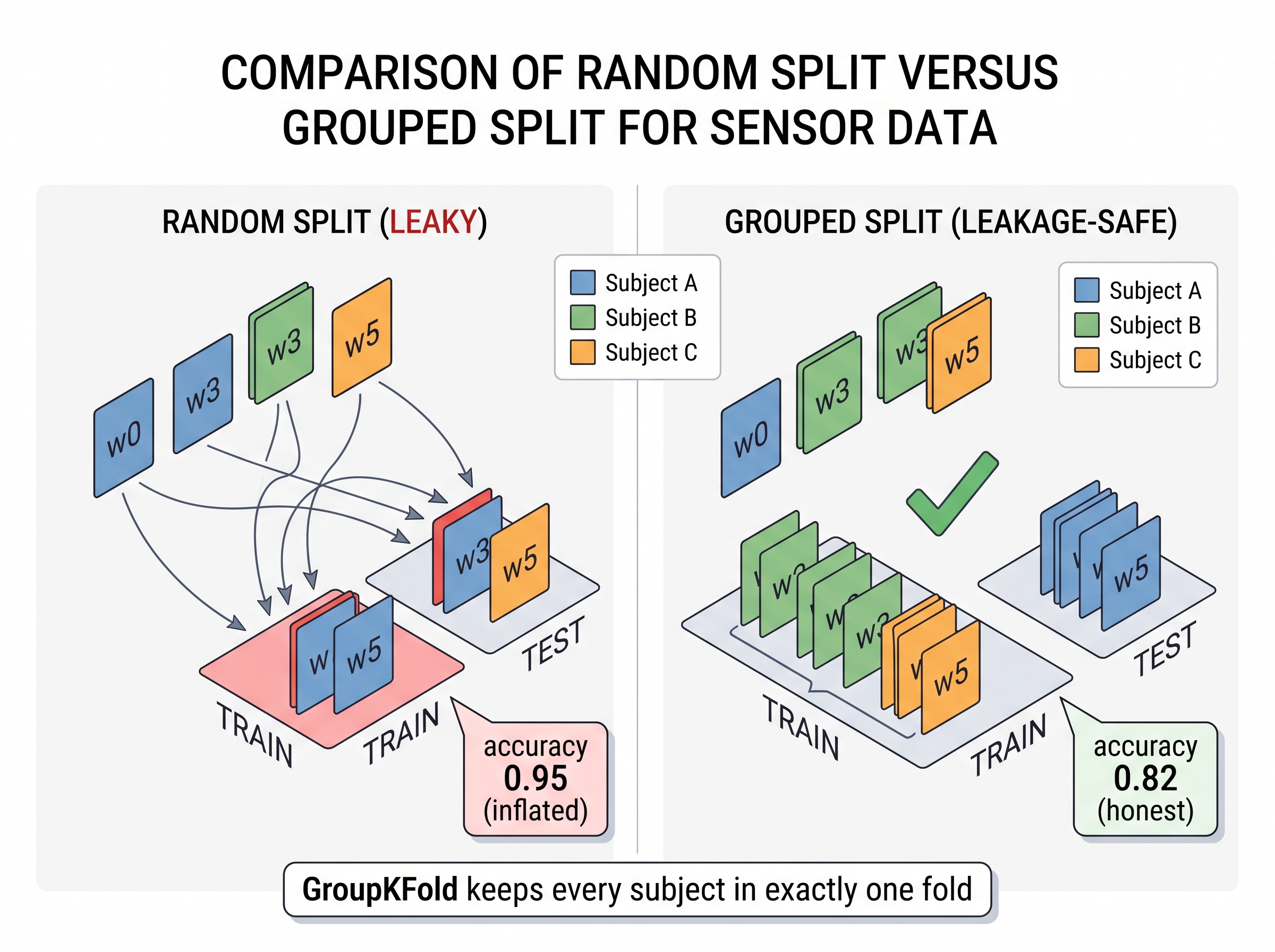
Random 3-fold. Shuffle indices, say to [w4, w1, w3, w0, w5, w2], then cut into three folds of two: test folds become {w4, w1}, {w3, w0}, {w5, w2}. Look at fold 1: its test set holds w1 (subject A) and w4 (subject C), while its training set holds w0 (subject A) and w5 (subject C). Subject A now sits on both sides, so the model can memorize A's resting-heart-rate bias from w0 and reuse it to score w1. Suppose the reported mean accuracy is 0.95.

Grouped 3-fold. GroupKFold assigns whole subjects to folds, never splitting a subject: fold 1 test = {A} = w0, w1; fold 2 test = {B} = w2, w3; fold 3 test = {C} = w4, w5. In every fold the tested subject is entirely absent from training, so no per-subject shortcut can leak. Suppose the reported mean accuracy is now 0.82.

Read-out. The gap 0.95 minus 0.82 equals 0.13, and that 13-point drop is exactly the leakage the random split was hiding: the same model, the same data, reported 95 percent one way and 82 percent the honest way, and only one of those numbers survives contact with a new subject. The number that survives grouped splitting is the one that predicts field performance on a subject the model has never seen.

How to hold the whole book in your head at once

Put the three pieces together and you hold a compact model of the entire volume. The verbs tell you what a chapter does, the level tags how deep it goes, the threads which cross-cutting concerns it must respect. Those three coordinates locate any chapter. Chapter 19, for instance, is an infer-and-represent chapter at level [R] that honors the calibration and leakage threads, and it teaches exactly that in Chapter 19, Time-Series Foundation Models. That is your mental table of contents. The rest of Part I fills in the measure foundations the other verbs stand on; from there you follow your own path across the arc until it converges, in the capstone, into one system.

What's Next

In Chapter 2, the arc begins for real with the first verb. That section opens up the measurement model \(x = h(s) + \eta\) and separates direct observables (what a sensor reports straight out) from indirect ones (what you must infer because the quantity you care about was never measured directly), the distinction that decides how much work every later verb has to do.