Sampling, latency, bandwidth, power, cost, and privacy as first-class constraints

"I could be accurate, cheap, fast, and private all at once. Pick three, and even three is me being generous with myself."

A Budget-Conscious AI Agent

What lets one sensing system run for years on a coin cell while another needs a wall socket to answer the very same question? Almost never the cleverness of the algorithm, and almost always the budget it has to fit inside. Section 1.5 walked the sensing chain from raw signal to decision as a sequence of stages; this section reads that same chain along a different axis: not what each stage does, but what each stage costs. We are deliberately not doing sampling theory here (that is the job of Chapter 3, Signals, Sampling, Time, and Synchronization); we are treating the sampling rate as one knob in a budget you cannot overspend. The only prerequisite is the notation from Section 1.3: a continuous signal \(x(t)\), its sampled form \(x[n]\), a hidden world state \(s\) we want to estimate as \(\hat{s}\), and the measurement model \(x = h(s) + \eta\). In short: fix the budget first and the deployment target hands you the model that fits inside it; accuracy only ranks what survives.

The six-constraint tension web

What the web contains: six quantities that every sensory-AI system spends. Sampling rate \(f_s\) sets how finely you observe \(x(t)\) in time and how many bits per second you generate. Latency is the delay from a physical event \(e\) at time \(t\) to the action \(a\) it triggers. Bandwidth is what your link (Bluetooth Low Energy or BLE, LoRa for Long Range, cellular, Controller Area Network or CAN bus) can actually carry off the node. Power is the energy budget, which on a coin cell or a harvested microwatt (energy scavenged from ambient light, vibration, or heat rather than drawn from a battery) is brutally finite. Cost is the per-node bill of materials (the total price of every component in one unit) and compute, multiplied by fleet size. Privacy is how much of the raw signal, and the identity latent inside it, ever leaves the sensor.

Latency, the term most often confused with bandwidth, is worth pinning down precisely: it is the wall-clock delay along the entire path from a physical event to the resulting action. That path sums sensing time, on-node compute, any transmission and queueing on the link, and remote compute plus the return trip. It matters because a control loop that acts too late acts on stale world state, so a fast-but-late estimate can be worse than useless (a braking decision that lands at 300 ms is a crash, not a slow success). Mechanically the delays add along the pipeline, whereas bandwidth only sets the transmission term. That is why a high-throughput link can still deliver painfully high latency. Budget by the tail (the 99th-percentile delay) rather than the mean whenever a missed deadline is unsafe. Reserve mean latency for soft, best-effort tasks such as background logging.

Engineers who treat these six as a checklist ship prototypes that pass on the bench and then flatten the battery or flood the radio the week they scale to the field, because the mechanism below was quietly linking every knob to every other one the whole time. Why they are a web and not a checklist: they are physically and economically coupled, so improving one degrades at least one other. Raising \(f_s\) improves your chance of catching a fast transient, but the raw data rate for a single channel is

where \(b\) is bits per sample and \(C\) is the channel count. Double \(f_s\) and you double the bytes the radio must send (bandwidth up), the energy per second the radio spends (power up), and, if you cannot afford to stream it all, the compute you must add on the node to summarize it (cost up). Every arrow in Figure 1 is a coupling of this kind. There is no operating point that maximizes all six; there are only Pareto-efficient trades (where a Pareto-efficient operating point is one you cannot improve on any constraint without giving up ground on at least one other), and picking one is a design decision, not a tuning afterthought.

How you reason with the web: fix the two constraints that are truly non-negotiable for your application first, then let the web tell you what the other four are allowed to be. A car's collision-braking system fixes latency and safety, so it accepts high cost and power. A soil-moisture sensor in a field fixes power and cost, so it accepts coarse sampling and long latency. When this matters most: at the very first architecture sketch, before a single line of model code, because the fixed constraints eliminate whole families of methods before you ever compare their accuracy.

No free lunch: accuracy, power, latency, and privacy trade against each other

If the budget chooses the model, its first and most consequential entry is a question of geography. The sharpest four-way tension lives in a single decision: where does the computation happen? Send raw \(x[n]\) to the cloud and a large model produces a high-accuracy \(\hat{s}\), but you have paid in bandwidth, in round-trip latency, in radio power, and, most consequentially, in privacy, because the raw signal (a face, a voice, a gait, a heartbeat) has now left the device and become someone else's liability. Run a compressed model on the node and you keep the raw signal local (privacy up), cut the round trip (latency down), and stop streaming (bandwidth and radio power down), but the smaller model is usually less accurate. That is the no-free-lunch structure: the same lever moves accuracy one way and moves privacy, latency, and power the other way. You do not get to opt out of the trade; you only get to choose where on the curve to sit.

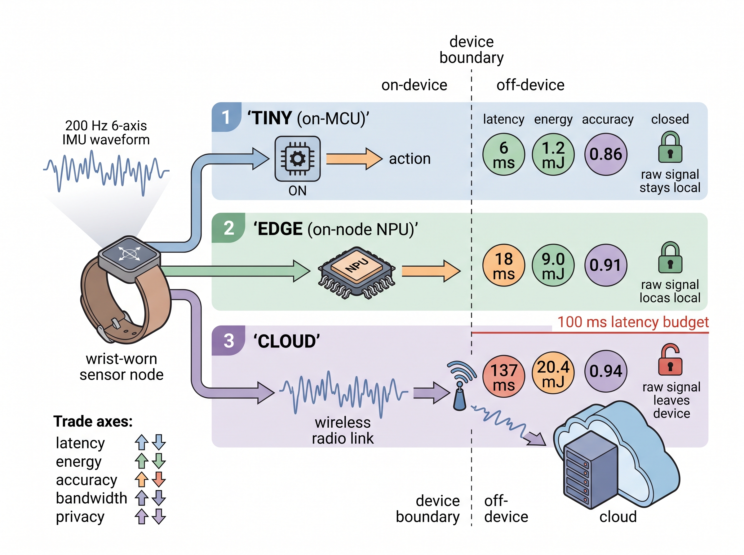
The short script below makes the trade concrete for one wearable design choice. It scores three placements of the same inference, cloud, edge, and a tiny on-device model, on a common latency and energy model, and reports which one respects a 100 ms latency budget while keeping the raw signal on the wrist. Figure 1.6.1 illustrates compute placement across the sensor-to-cloud boundary (tiny on-device vs edge vs cloud) and how each placement trades latency, energy, accuracy, bandwidth, and privacy.

import numpy as np

# One 6-axis IMU window: 200 Hz, 2 s, float32
fs, seconds, channels, bytes_per = 200, 2.0, 6, 4
payload_bytes = int(fs * seconds * channels * bytes_per)  # raw window

# Simple, defensible per-option models (latency ms, energy mJ, keeps raw local?)
def cloud():
    tx_ms = payload_bytes * 8 / 1e6 * 1e3      # 1 Mbit/s effective uplink
    return dict(latency=tx_ms + 60, energy=payload_bytes * 8 * 5e-6 + 20,
                local=False, acc=0.94)
def edge():
    return dict(latency=18, energy=9.0, local=True, acc=0.91)   # NPU on-node
def tiny():
    return dict(latency=6, energy=1.2, local=True, acc=0.86)    # MCU model

BUDGET_MS = 100
for name, opt in [("cloud", cloud()), ("edge", edge()), ("tiny", tiny())]:
    ok = "PASS" if opt["latency"] <= BUDGET_MS and opt["local"] else "fail"
    print(f"{name:5s}  lat={opt['latency']:6.1f} ms  "
          f"E={opt['energy']:5.1f} mJ  acc={opt['acc']:.2f}  "
          f"local={str(opt['local']):5s}  [{ok}]")

Read Listing 1 as a decision, not a benchmark. The cloud model is the most accurate at \(0.94\), yet it fails the actual requirements: its round trip blows the latency budget and it ships the raw signal off-wrist. Between the two survivors, the choice is a pure trade of five accuracy points for a roughly \(7\times\) energy saving, which on a coin cell can mean weeks of extra battery life. The constraint did not rank the models by accuracy; it deleted the most accurate one and handed you a smaller menu.

import tensorflow as tf
conv = tf.lite.TFLiteConverter.from_saved_model("model/")
conv.optimizations = [tf.lite.Optimize.DEFAULT]   # int8 quantization
open("model_int8.tflite", "wb").write(conv.convert())

Cost per node dominates at fleet scale and caps model size

Everything so far has weighed a single device; multiply that device by a fleet and a new constraint quietly overtakes the rest. What changes at scale: a single prototype hides the constraint that eventually dominates. When you ship one clever device, you can afford a fast processor and a generous battery. When you ship \(N\) of them, every dollar and every milliwatt is multiplied by \(N\), and the total system cost is roughly

where each per-node term is small but \(N\) is large. Why this caps model size: the cheapest microcontroller that meets the requirement sets the per-node compute budget. At a fleet of a million nodes, a one-dollar processor upgrade becomes a million-dollar line item. That single sourcing decision fixes the flash, the RAM, and the clock, which in turn cap the number of model parameters you can store and the inference you can run per sample. The model does not size the hardware; the fleet economics size the hardware, and the hardware sizes the model.

Privacy as a design constraint that relocates computation

Cost prunes the design tree by economics; privacy prunes it by rule, and the second cut is often the sharper of the two. Privacy is the constraint most often mistaken for a checkbox, a consent form signed after the architecture is frozen. Treated that way, it is powerless. Treated as a first-class engineering constraint, it is one of the strongest forces in the web, because it does something the others cannot: it dictates where computation is allowed to happen. If a rule says the raw signal must never leave the device (a face, a voice print, an electroencephalography (EEG) trace, a continuous heart rhythm), then cloud inference is not a slower option to be weighed on a curve; it is off the table. The privacy constraint has pruned an entire branch of the design tree before accuracy is ever discussed.

This is why privacy foreshadows so much of the book's back half. Keeping the raw signal local forces computation onto the edge (Chapter 59). Learning from a fleet without collecting anyone's raw data forces federated training, where nodes share model updates instead of measurements. Sensing on harvested energy with no persistent store forces batteryless designs that are private almost by construction because there is nothing durable to exfiltrate. In each case privacy did not sit on top of the architecture; it relocated the computation and thereby chose the architecture. The regulatory and ethical framing of that choice, and the standards that increasingly make it mandatory rather than optional, are developed in Chapter 70, Responsible Sensory AI and Regulation.

Constraint-driven design: the deployment target chooses the method

Pulling the threads together yields one reorienting habit: do not start from the model and defend it against the constraints; start from the constraints and let them nominate the model. Write down the two constraints your application cannot move (latency and safety for the braking system, power and cost for the soil sensor, privacy and battery life for the wearable electrocardiogram (ECG)). Those two fixed points collapse the tension web to a small feasible region that usually holds one obvious method and a couple of runners-up. Accuracy then ranks only those survivors. That is what "the deployment target chooses the method" means: by the time you compare accuracy numbers, the constraints have already done most of the choosing. Much of this book is a catalog of which methods survive which constraint budgets, which is why we return to this web whenever a new technique promises accuracy without naming its price.

What's Next

In Section 1.7, we turn from the constraints that shape any sensory-AI system to the shift reshaping how we build them: the 2023 to 2026 move from bespoke, hand-tuned pipelines toward foundation models and agentic sensing, and what that shift does, and does not, do to the six-constraint web you just met.