"First I sorted the sensors by what they measure, then by how fast, and then I had a spreadsheet, and a spreadsheet I can finally understand."
A Taxonomically Inclined AI Agent
The big picture
The sensor world looks like a zoo: an accelerometer sampling a wrist at 50 Hz sits next to a lidar spinning out a million 3D points per frame, next to an electrode reading microvolts off the scalp. The trap is to study each device as its own island. This section builds two orthogonal maps instead. One axis catalogs a modality by four physical properties: what quantity it transduces, how fast it samples, its spatial and channel dimensionality, and the structure of its output. The other axis catalogs the task family we ask of it. Cross them and you get a matrix in which a single recipe reappears across wildly different hardware. That matrix is the planning artifact you will fill in directly in Lab 1, and it is the reason the rest of this book can teach six verbs (measure, clean, represent, infer, fuse, deploy) rather than seventy-two device manuals.
How can the same twenty lines of code that flag a failing bearing also flag an abnormal heartbeat? The answer is that both sit at the same address on a two-axis map, and this section builds that map using only the four quantities introduced in Section 1.3: the raw signal \(x(t)\), the hidden world state \(s\), the discrete event \(e\), and the action \(a\). If those symbols are unfamiliar, read that section first; everything here is a way of organizing them. Deployment constraints such as latency, power, and privacy belong to Section 1.6, and the pipeline stages that turn \(x\) into \(a\) belong to Section 1.5. This section answers only what kind of thing a sensor is and what kind of question we pose to it.
Four axes that pin down any modality
A modality is not defined by its brand or its bus. It is defined by where it sits along four axes, and those four coordinates predict almost everything about how you will process it. Figure 1.4.1 illustrates the four modality axes as a sensor feature vector.
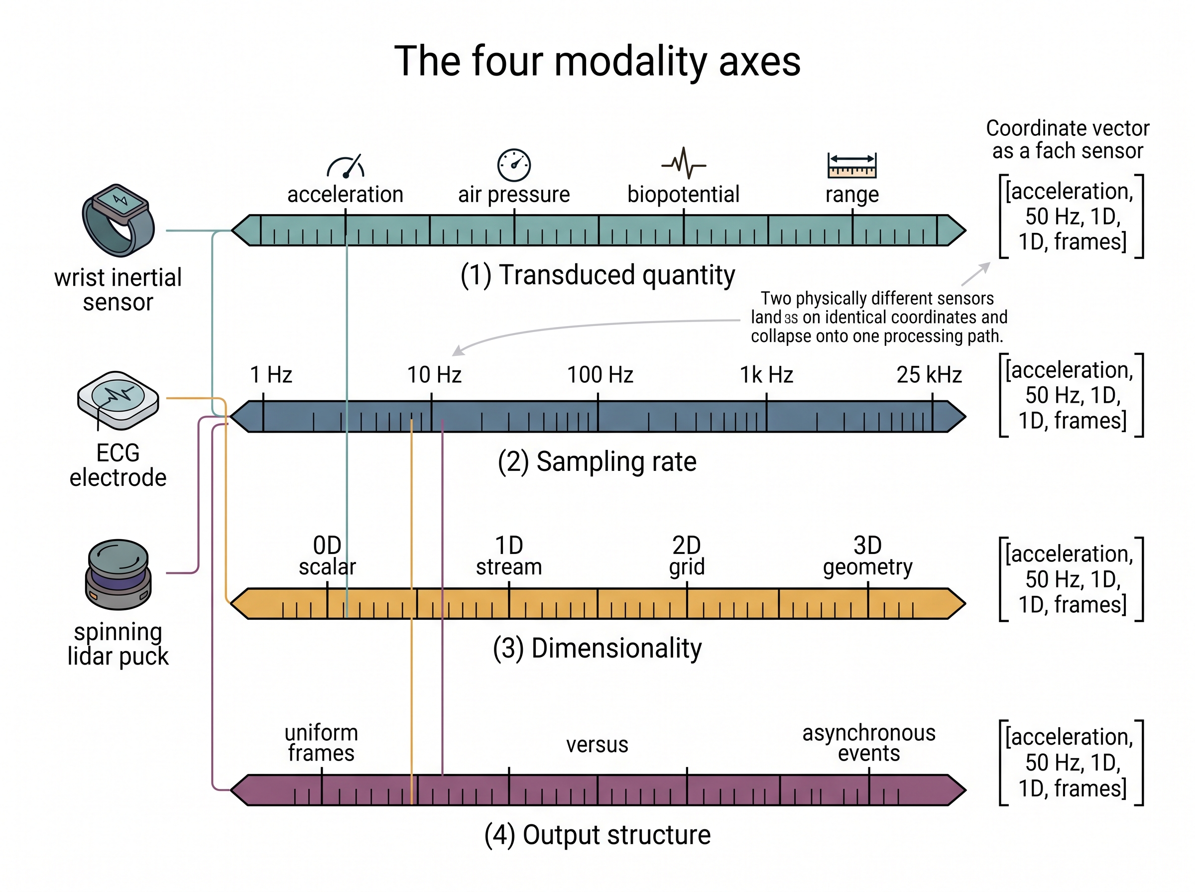
Transduced quantity: what physics is being measured. Every sensor is a function \(x = h(s) + \eta\) that maps some hidden state \(s\) to a signal through a response \(h(\cdot)\) with noise \(\eta\). The first question is what \(s\) actually is. An accelerometer transduces proper acceleration; a microphone transduces air pressure; a photodiode transduces irradiance; an electrocardiogram (ECG) electrode transduces the body-surface potential of cardiac depolarization. This choice fixes the noise physics you will fight in Chapter 2. Thermal noise, shot noise, and motion artifact are not interchangeable, and knowing the transduced quantity tells you which one dominates.
Sampling rate: how fast the world is queried. A signal sampled at rate \(f_s\) can only faithfully represent content below \(f_s/2\); above that, energy folds back as aliasing (the sampling theorem, developed in Chapter 3). Human activity lives comfortably at tens of hertz, so wrist inertial sensors run at 25 to 100 Hz. Audio needs kilohertz. An ECG at 250 to 500 Hz resolves the sharp QRS complex (the tall, narrow spike in each heartbeat that marks the ventricles contracting); an electroencephalogram (EEG) event of interest may demand more. Sampling rate sets your window length, your memory budget, and whether a Fourier view even makes sense.
Aliasing is the specific failure that bound guards against. It is the irreversible corruption that appears when signal energy above \(f_s/2\) reaches the converter anyway, and it matters because no later filtering can undo it once the samples are stored. The mechanism folds, or mirrors, the too-fast content back down into the low frequencies. There it masquerades as a genuine low-frequency component, and you can no longer separate it from the real thing. When the sensor's rate is fixed and you cannot raise \(f_s\), insert an analog anti-alias low-pass filter before the converter. When you control the rate, sampling faster than twice the highest frequency of interest is the cleaner remedy.
Checkpoint
So far: two of the four modality axes are set (the physical quantity a sensor transduces and how fast it samples), and we have seen why sampling too slowly causes irreversible aliasing. The remaining two axes, dimensionality and output structure, come next.
From time to space: shape and structure
Rate settles the temporal grain of a signal; the third axis turns from time to space. Dimensionality: spatial extent and channel count. A thermistor is a scalar time series (zero spatial dimensions, one channel). A tri-axial accelerometer is three channels of a point. A camera frame is a 2D grid with three color channels. A lidar sweep is an unordered set of 3D points. This axis decides your architecture: 1D convolutions and recurrent models for streams, 2D convolutions or vision transformers for grids, and point-set or graph networks for the geometry covered in Chapter 40.
Output structure: how samples are organized in time. Some sensors emit uniformly clocked frames. Others, such as event cameras, emit asynchronous, sparse spikes only when something changes, so there is no fixed \(f_s\) at all. Structure determines whether you can stack a tensor of shape (time, channels) or must reason over irregular timestamps. In short: pin a sensor to four coordinates and its question to one of six task families, and you stop writing seventy-two device manuals and start reusing one recipe per cell.
Key insight
The four modality axes are not a filing convenience; they are a feature vector for the sensor itself. Two devices with nothing physically in common, a hydrophone and a strain gauge, become the same processing problem once you notice they share coordinates: scalar quantity, kilohertz sampling, one channel, uniform frames. That collapse is exactly why one denoising or forecasting method can serve dozens of instruments. You classify the sensor so you can reuse the software.
Mental Model
Think of the counter at an international shipping office. The clerk never asks whether your box holds paperback books, ceramic mugs, or dried mangoes; the parcel is priced and routed from four numbers alone: its weight, its outer dimensions, its declared fragility, and its destination zone. Two shipments with nothing in common inside follow the identical handling path the instant those four numbers match. The modality axes are exactly that shipping label for a sensor: quantity, rate, dimensionality, and output structure are the numbers, and any two devices whose numbers agree drop onto the same processing conveyor no matter what physics is packed inside the box.
Six task families that recur everywhere
The second axis is the question. Across every modality, the inference targets collapse into six recurring families, each defined by the type of its output rather than by the domain.
- Classification. Map a window to one label from a fixed set: \(x[n] \mapsto c \in \{1,\dots,C\}\). "Walking vs running", "arrhythmia vs sinus rhythm".
- Regression and forecasting. Map to a continuous quantity, either now (estimate current heart rate from photoplethysmography (PPG)) or ahead in time (forecast \(x_{k+1{:}k+H}\) from \(x_{1{:}k}\)). The forecasting variant is the province of Chapter 19.
- Detection. Localize discrete events \(e\) in time (or space): find when a footstep, a keyword, or a machine fault onset occurs, not just whether the window contains one.
- State estimation. Recover a continuous latent \(\hat{s}_t\) that evolves over time, typically with a dynamics model: orientation, position, battery charge. This is the Kalman and Bayesian-filtering territory of Part III.
- Segmentation. Assign a label to every sample (temporal) or every pixel or point (spatial), partitioning the signal into contiguous regions.
- Anomaly detection. Flag samples that depart from a learned notion of normal, usually without labeled examples of the failure. Central to condition monitoring.
These families are not exclusive. Human activity recognition, treated in depth in Chapter 26, is windowed classification when you want a label per two-second clip, but temporal segmentation when you want exact transition boundaries. Naming the family is the first design decision, because it fixes the loss function, the metric, and the label format long before you pick a model.
Common Misconception
A common misconception is that each sensor "belongs" to one task, that a camera is inherently for classification and an accelerometer is inherently for activity recognition, as if the modality picks the column for you. The two axes are orthogonal: any modality can be posed against any task family, and the very same accelerometer legitimately answers a classification, a regression, a detection, or an anomaly question depending only on what you choose to ask, not on the hardware.
In practice: one gearbox, four questions
A wind-turbine operator instruments a gearbox with a single accelerometer sampling at 25.6 kHz (a scalar quantity, kilohertz sampling, one channel, uniform frames). From that one modality the maintenance team poses four different task-family questions. Is the current state healthy or degraded? is classification. How many operating hours remain before the bearing fails? is regression, specifically remaining-useful-life prediction. At what instant did the impact signature first appear? is detection. Does today's vibration spectrum look unlike every healthy day we have on record? is anomaly detection, and it is typically the one that ships first, because it needs no examples of the fault. Same sensor, same bytes on the wire, four columns of the matrix, four different pipelines downstream.
The modality-by-task matrix
Get this cross wrong and device teams often quietly rebuild the same detector from scratch, several times over, each one blind to the others who already solved it. Cross the two axes and you get the organizing artifact of this section: a grid whose rows are modalities and whose columns are task families. Each cell names the canonical question people actually ask of that pairing. The matrix in the table below is a small slice; the point is not to be exhaustive but to show that the columns are the same no matter how alien the rows look to each other.
| Modality | Classification | Regression / forecasting | Detection | Anomaly detection |
|---|---|---|---|---|
| Wrist inertial measurement unit (IMU) (50 Hz, 6-ch, frames) | Activity type | Energy expenditure | Fall onset | Atypical gait |
| ECG (360 Hz, 1-ch, frames) | Arrhythmia class | Heart-rate trend | R-peak timing | Novel morphology |
| Microphone (16 kHz, 1-ch, frames) | Keyword | Sound level forecast | Gunshot onset | Rare acoustic fault |
| Lidar (10 Hz, 3D point set) | Object category | Track velocity | Obstacle appearance | Sensor dropout |
| Vibration (25.6 kHz, 1-ch) | Health state | Remaining useful life | Impact instant | Off-manifold day |
Read the table by columns and the recurrence stands out. The "anomaly detection" column poses one statistical question, is this point off the learned manifold of normal (the manifold being the low-dimensional surface that healthy data traces out inside the space of all possible signals), whether the point is a gait cycle, a heartbeat, or a bearing spectrum. A method invented for one row therefore transfers to the next, and a single foundation model can increasingly serve a whole column, dozens of physically unrelated instruments answered by one frozen backbone (the term is made concrete in the Research Frontier note just below). Read the table by rows and you get the planning template for Lab 1: place each dataset you survey in exactly one row-and-column cell, then annotate three cross-cutting properties the matrix alone does not capture.
Research Frontier
The "one model per column" idea turned concrete in 2024. MOMENT (Goswami et al., ICML 2024) is a family of open time-series foundation models pre-trained on a broad "Time-Series Pile" that handles classification, forecasting, imputation (filling in missing samples), and anomaly detection from a single frozen backbone, and Amazon's Chronos (Ansari et al., 2024) tokenizes raw values so a language-model architecture forecasts sensors it never saw, zero-shot (as of 2024, Amazon's faster Chronos-Bolt variant has largely superseded the original for practical deployment). Both push past this section's one-method-per-cell framing toward a single pre-trained model that spans an entire task-family column across modalities absent from its training set.
Real-World Application: industrial condition monitoring
Amazon Lookout for Equipment is a managed service that reads the anomaly-detection column of this matrix for arbitrary industrial hardware: a customer streams pumps, motors, or compressors as raw multichannel time series, and one learned notion of normal flags off-manifold behavior without a single labeled fault. It works largely because, in practice, the anomaly question does not care whether the row is a vibration channel or a temperature loop, so the same backbone serves a plant full of physically unrelated sensors.
Fun note
The zoo metaphor is only half a joke. A working sensor lab really does contain wildly different animals in adjacent cages, and the natural instinct is to hire a specialist per species. The taxonomy is what lets one keeper feed them all: once you accept that a heartbeat and a bearing fault are the same anomaly-detection problem wearing different fur, the staffing plan changes.
Three cross-cutting properties the matrix does not show
A cell tells you the shape of the question. It does not tell you how hard the data will be to work with. Three additional properties, which you will record for every dataset in Lab 1, cut across all cells.
Noise source. The \(\eta\) in \(x = h(s) + \eta\) is not generic. Wearable inertial data is dominated by motion artifact and loose-contact dropouts; ECG fights baseline wander and mains interference; lidar suffers from reflectivity and range dropout. Knowing the dominant noise source picks your cleaning strategy in Part II.
Label cost. Some labels are nearly free (a machine's own controller logs when it faulted). Others require a clinician-adjudicated gold standard at real per-sample expense. High label cost is precisely what pushes a project toward self-supervised (learning from unlabeled data by predicting one part of a signal from another) and foundation-model approaches, and it is the reason anomaly detection, which needs no fault labels, is so often the first thing to ship.
Deployment constraint. A model that must run on a coin-cell wearable faces different limits than one on a vehicle compute stack. We only tag this property here; Section 1.6 promotes latency, bandwidth, power, cost, and privacy to first-class citizens.
Reading a dataset into the taxonomy, in code
With those three cross-cutting properties noted for later, the four core axes are the part a program can compute directly. The taxonomy is meant to be operational, not decorative. The short script below encodes each modality as its four-axis coordinate and prints the compact "sensor feature vector" you will build a spreadsheet of in Lab 1. It is the seed of that survey: given raw metadata, it classifies the sensor before a single sample is processed.
import pandas as pd

# Each row is one modality described by the four taxonomy axes.
sensors = pd.DataFrame([
    #  name,            quantity,        f_s_hz, channels, spatial_dims, output
    ["wrist_imu",      "acceleration",     50,       6,        0,     "frames"],
    ["ecg_lead",       "biopotential",    360,       1,        0,     "frames"],
    ["microphone",     "air_pressure",  16000,       1,        0,     "frames"],
    ["lidar",          "range",            10,       1,        3,     "point_set"],
    ["event_camera",   "log_irradiance",   -1,       1,        2,     "async_events"],
], columns=["name", "quantity", "f_s_hz", "channels", "spatial_dims", "output"])

def nyquist(f_s):
    return "asynchronous" if f_s < 0 else f"{f_s / 2:.0f} Hz usable band"

sensors["max_content"] = sensors["f_s_hz"].apply(nyquist)
sensors["shape_class"] = sensors["spatial_dims"].map({0: "stream", 2: "grid", 3: "geometry"})

print(sensors[["name", "quantity", "max_content", "shape_class", "output"]].to_string(index=False))nyquist and shape_class helpers turn raw metadata into a printed sensor feature vector; a negative sampling rate flags an asynchronous, event-structured stream that has no fixed Nyquist band.Notice what the code makes visible. The event camera has no meaningful \(f_s/2\) because it is not clocked at all, so its usable band prints as asynchronous. Spatially it is still a 2D grid, the same shape class as an ordinary frame camera, yet its output structure is async_events rather than uniform frames. That contrast is why "output structure" earns its place as a full axis rather than a footnote to sampling rate: it is the coordinate that separates an event camera from a frame camera that matches it on every other number.
Right tool: let a loader read the axes for you
Hand-typing sampling rate and channel count is fine for five sensors and error-prone for fifty. For real recordings, formats such as the European Data Format (EDF) for biosignals and WAV for audio store these axes in their headers, so a loader recovers them in one call.
import soundfile as sf
x, f_s = sf.read("machine.wav")          # samples, sampling rate
channels = 1 if x.ndim == 1 else x.shape[1]
print(f_s, channels, x.shape[0] / f_s, "seconds")soundfile. The single sf.read call returns both the samples and the sampling rate, and the array shape yields the channel count, so the rate and dimensionality axes are read rather than hand-typed.Three lines replace roughly a dozen lines of manual header parsing and unit bookkeeping, and the library handles endianness, bit depth, and multi-channel interleaving internally. You still decide the task family; the library only recovers the modality axes.
The figure below plots the two axes as a plane. Any sensing project is a single point on it: pick a modality row and a task column to locate your problem in the territory this book spends fourteen parts mapping.
Try It: Place a real recording on the taxonomy grid
With a laptop and the standard scientific-Python stack, you can walk one file from raw bytes to a single matrix cell in about fifteen minutes.
- Install the tools and grab a clip: run
pip install soundfile numpy, then save a few seconds of audio asclip.wav(a phone voice memo exported to WAV works fine). - Recover the modality axes from the header: load with
x, f_s = soundfile.read("clip.wav"), then write down the four coordinates (quantity = air pressure, rate =f_s, channels =1 if x.ndim == 1 else x.shape[1], output = uniform frames) and print the usable bandf_s / 2. - Pick one task-family column and state what it commits you to: for classification, name the label set and a cross-entropy loss; for anomaly detection, name a score that needs no labels at all.
- Implement the anomaly column cheaply: split
xinto 50 ms frames, compute each frame's energy, and flag frames whose energy z-score (its distance from the mean in units of standard deviation) exceeds 3 as candidate events. - Confirm the reuse claim: swap only the input, feeding an IMU or ECG column loaded from a CSV, leave the framing-and-z-score code untouched, and watch the identical detector run on a completely different modality.
Step-Through: the energy z-score anomaly detector
Trace the frame-energy detector from the Try It box on tiny, concrete numbers so you can see every arithmetic step, not pseudocode. Suppose you have already computed one energy value per frame for four quiet baseline frames: 0.10, 0.12, 0.08, 0.10. Then a fifth frame arrives with energy 0.50, and you must decide whether it is an event.
- Baseline mean. Average the four normal frames: (0.10 + 0.12 + 0.08 + 0.10) / 4 = 0.40 / 4 = 0.10.
- Baseline deviations. Subtract that mean from each: 0.00, +0.02, -0.02, 0.00.
- Baseline standard deviation. Square the deviations (0, 0.0004, 0.0004, 0), average them (0.0008 / 4 = 0.0002), and take the root: sqrt(0.0002) = 0.01414.
- Score the new frame. The z-score of energy 0.50 against that baseline is (0.50 - 0.10) / 0.01414 = 0.40 / 0.01414 = 28.3.
- Threshold. Since 28.3 exceeds the cutoff of 3, the frame is flagged as a candidate event. Had the new frame carried energy 0.11 instead, its z-score would be (0.11 - 0.10) / 0.01414 = 0.71, comfortably below 3, and it would pass as normal.
The whole detector is just those five arithmetic steps, and nothing in them mentions audio. Feed it accelerometer frame energies and the identical numbers run: that is the reuse claim made concrete.
Lab: one detector, three modalities
Goal. Confirm empirically that a single anomaly-detection method (this section's core reuse claim) transfers unchanged across three physically unrelated modality rows of the matrix.
Tools needed. Python with numpy, scipy, and soundfile (pip install numpy scipy soundfile). Three short real recordings, one per modality: an audio clip (a phone voice memo exported to WAV), an accelerometer trace (one axis of any UCI Human Activity Recognition CSV, or a phone-logger export), and an ECG strip (a lead from the MIT-BIH sample records loaded with wfdb, or any single-column CSV). A few seconds of each is plenty.
Procedure. Write one function frame_zscore(signal, frame_len, thresh) that splits the 1D signal into non-overlapping frames, computes each frame's energy (sum of squares), z-scores those energies against the recording's own mean and standard deviation, and returns the indices whose z-score exceeds thresh. Call it on all three signals without editing a line of the function between calls.
What to vary. Sweep thresh across 2, 3, and 4, and try two frame lengths (for example 50 ms and 200 ms worth of samples, computed from each recording's own f_s).
What to observe. Record how many events each modality yields at each setting. You should see the identical code run on all three, the flagged-event count fall as the threshold rises, and the frame length trade temporal precision against noise robustness. The takeaway to write down: you located three different rows of the taxonomy matrix, posed the same column (anomaly detection) against all of them, and shipped one implementation for the whole column.
Exercise
A smart-building team deploys a passive-infrared (PIR) occupancy sensor that outputs a single binary channel updated at 1 Hz. (a) Give its four modality-axis coordinates. (b) The team wants to know how many people will be in a room fifteen minutes from now. Which task family is that, and why is it not classification? (c) Name the one cross-cutting property most likely to block a supervised approach here, and justify your choice in one sentence.
Self-check
1. Why is "output structure" a separate modality axis rather than a special case of sampling rate?
2. Two sensors share all four modality coordinates but you would still process them very differently. Name a cross-cutting property that could explain the divergence.
3. In the gearbox example, which task family ships first in practice, and what property of the labels makes that possible?
What's Next
In Section 1.5, we stop asking what kind of thing and start tracing how it flows: the sensing chain that carries a raw signal \(x(t)\) through conditioning, representation, and inference to an action \(a\). The taxonomy you built here becomes the labels on the chain's input; the next section connects those inputs to the six verbs that structure the whole book. A fuller catalog of the datasets referenced throughout, with their axes pre-tabulated, lives in Appendix E: Datasets and Benchmarks.