"In text I could always scroll back and reread. Out here, the instant I hesitate, the instant is already gone."
A Newly Embodied AI Agent
The line this book is built on
Most of modern machine learning was shaped by two data sources: text scraped from the web and pixels scraped alongside it. Both are authored artifacts. A human wrote the sentence; a camera and an editor chose the photo. Sensory AI draws from a different well. Its data is generated by physics, sampled by an instrument, and stamped with an instant that will never recur. This section draws the sharp line between the two worlds and enumerates the consequences of that difference. Every one of them is a reason a method that dominates a language benchmark can quietly fail on a stream of accelerometer samples.
Section 1.1 introduced the sensor as an imperfect window on the world. Here we do not re-litigate sensor imperfection; we take it as given and ask a sharper question: what changes about the practice of building AI when your inputs come from an instrument rather than a corpus? We use the book's notation throughout: the hidden world state is \(s\) (or \(s_t\) over time), the raw transduced signal is \(x(t)\), the sampled signal is \(x[n]\) or \(x_k\), the conditioned observation a model consumes is \(y\), and the measurement model is \(x = h(s) + \eta\). If any of these look unfamiliar, the notation is laid out in full in this chapter's front matter and in Chapter 2.
Measurement versus retrieval: where the data comes from
A language model is trained on a fixed set of documents. Every token it will ever see at training time already exists, sitting in a file, and can be shuffled, deduplicated, re-tokenized, and revisited an arbitrary number of times. The generative process is authorship: a human decided what to write. When the model later needs more of a document, it retrieves it. The data is a library.
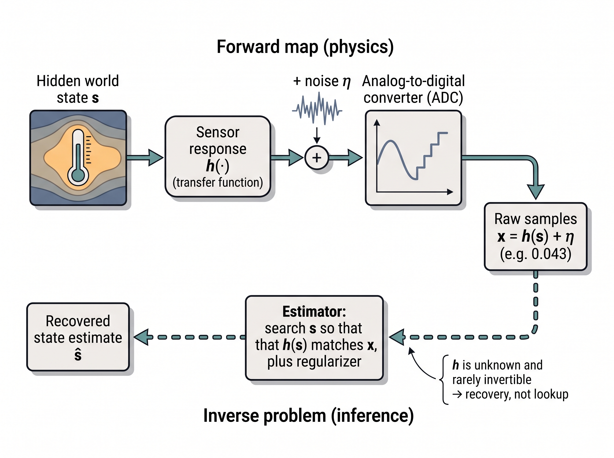
Get this one mapping wrong and the failure is not a typo but a false belief about the world: a navigation filter that places a car a full lane over, or a pulse oximeter that reads a comfortable 98 percent while a patient is quietly desaturating. A sensor produces data by a fundamentally different process. A physical quantity drives a transducer that maps state to a voltage: temperature, acceleration, photon flux, the electrical potential across a patch of skin. Then an analog-to-digital converter (ADC) turns that voltage into numbers. Formally this is the measurement model \(x = h(s) + \eta\): the true state \(s\) passes through the sensor response \(h(\cdot)\) and picks up noise \(\eta\). No human authored the number 0.043; the world did, through a transfer function (the fixed input-to-output relationship of the sensor). This has an immediate consequence that has no analogue in text. The mapping \(h\) is not the identity and is rarely even known exactly, so recovering \(s\) from \(x\) is an inverse problem, not a lookup. In text the signal is the meaning; in sensing the signal is evidence about a hidden cause you must infer.
To make that word precise: an inverse problem is the task of recovering an unknown cause \(s\) from measured effects \(x\) when only the forward map \(h\) that turns causes into effects is known, and it matters because almost every sensory estimate, from position to core temperature to heart rate, is one in disguise, so getting it wrong means confidently reporting a state the world never occupied. Mechanically you solve it by assuming a model of \(h\), then searching for the \(s\) whose predicted measurement \(h(s)\) best matches what you actually observed, usually with a regularizer that keeps the answer stable when many candidate states explain the data almost equally well. Reach for an explicit inverse-problem formulation whenever \(h\) is non-trivial, poorly conditioned (so that small measurement errors translate into large errors in the recovered state), or noisy; when \(h\) is close to the identity and the noise is small, a direct calibration lookup is cheaper and entirely sufficient. Figure 1.2.1 illustrates The measurement model as a forward-and-inverse pipeline (x = h(s) + noise).
Checkpoint
So far: a sensor turns a hidden physical state \(s\) into numbers through a noisy, imperfect map \(x = h(s) + \eta\), so recovering \(s\) is an inverse problem you have to solve, not a value you can look up. The rest of this section works through the practical consequences of that one fact.
Units, calibration, and dimensional analysis
Inferring that hidden cause presumes you already know what physical quantity the measurement stands for, which is the next thing a corpus never forces you to track. Every sensor reading carries physical units. A token does not. This sounds like bookkeeping until it changes an answer. Suppose two accelerometers report a peak of 2.0. One is scaled in \(g\) (multiples of gravity), the other in \(\mathrm{m/s^2}\). They differ by a factor of 9.81, and a fall detector that confuses them will either fire on a brisk sit-down or sleep through a genuine collapse. There is no equivalent failure in a token stream, because tokens are dimensionless indices into a vocabulary; you cannot accidentally feed a model "meters" where it expected "seconds."
Units also gate a tool text people never need: calibration. A raw count from an ADC is related to a physical quantity by parameters that drift per unit and per day. A thermistor's resistance-to-temperature curve, an inertial measurement unit (IMU)'s bias and scale factor, a pulse oximeter's absorption coefficients: these are estimated, stored, and reapplied. The conditioned observation \(y\) that your model actually consumes is often \(y = c(x)\) for some calibration map \(c\) that undoes part of \(h\). Skipping calibration does not produce a slightly worse model; it produces a model that learned one device's idiosyncrasy and cannot transfer to the next unit off the line. Dimensional analysis, the discipline of checking that both sides of an equation carry the same units, is a free correctness test that in practice catches sensor-pipeline bugs a unit test suite would miss. In short: a corpus stores answers; an instrument only ever hands you evidence.
Let a units library carry the dimensions
You can track units by hand with naming conventions and prayer, or you can attach them to the quantities themselves and let arithmetic enforce dimensional consistency. A hand-rolled checker with per-quantity guards is easily 30 or more lines and still misses cases. A units library collapses that to three:
import pint
u = pint.UnitRegistry()

peak = 2.0 * u.g                      # acceleration in multiples of gravity
threshold = 25.0 * u("m/s**2")        # a fall threshold expressed differently
is_fall = peak.to("m/s**2") > threshold # auto-converts; raises if units are incompatiblepint units to a fall threshold so a 2.0 g peak is auto-converted before the comparison, turning a mixed-unit acceleration-versus-threshold test into a checked operation that raises rather than silently mis-fires.The library handles unit conversion, dimensional compatibility checks, and a registry of International System of Units (SI) base and derived units internally, and it raises an error the instant you compare an acceleration with a velocity. That single guard turns a class of silent numeric bugs into a loud exception at the line where the mistake happens.
The arrow of time: causality and the online constraint
Units settle what each sample means, but they say nothing about when you are permitted to use it, and here physical data imposes a limit a corpus never does. A corpus has no privileged direction of time. You can read the last page first, and standard training happily attends both left and right, because every token co-exists in the same file. Physical data is different in a way that is easy to state and easy to violate: at time \(t\) you have access only to samples up to \(t\). The future has not happened. Any estimate \(\hat{s}_t\) that a deployed system produces must be a function of \(x_{k}\) for \(k \le t\) only. This is the causal, or online, constraint, and it is not a stylistic preference; it is physics.
The trap is that this constraint is invisible during offline development, where the whole recording sits in a NumPy array and slicing forward is one keystroke away. A smoother that averages a window centered on the current sample, a normalizer that subtracts the whole-recording mean, a label assigned by peeking a few samples ahead: each leaks future information and inflates offline accuracy, then collapses in deployment where that future does not exist yet. This is temporal leakage, and it is in practice one of the most common ways sensor projects report a number they can never reproduce in the field. We treat it as a first-class hazard in Chapter 5 on leakage-safe datasets, and it reshapes model design too: it is the reason architectures with a lookahead-free structure matter for streaming, a thread picked up in Chapter 19 on time-series foundation models.
Research Frontier
The large-model recipe that reshaped text is now being pointed at raw sensor streams. Chronos (Ansari et al., 2024, "Chronos: Learning the Language of Time Series") quantizes real-valued measurements into a fixed vocabulary and pretrains a T5-style language model on them, and TimesFM (Das et al., 2024, "A decoder-only foundation model for time-series forecasting") pretrains on hundreds of billions of time points to forecast zero-shot on series it never saw in training. These systems bring transfer learning to signals that used to demand a bespoke model per deployment, but they do not repeal the constraints this section names: a forecasting foundation model is only deployable online if its context is strictly causal, and it still inherits the non-stationarity of the instrument that produced the stream. The frontier question is how to keep a pretrained time-series model calibrated as the hardware drifts, which the field is only beginning to address.
Figure 1.2.1 makes the contrast concrete. On the left, bidirectional arrows into a fixed corpus; on the right, a clock that only moves forward and a boxed future the model cannot touch.
Step-Through: causal versus whole-recording normalization
Trace both normalizers on a tiny five-sample recording \(x = [1,\,2,\,9,\,3,\,4]\), where the spike at index 2 is the event we want to keep visible. We normalize the sample at index 2.
Whole-recording (non-causal) z-score. A z-score rescales a value by subtracting a mean and dividing by a standard deviation. Use every sample, including the two future ones. Mean \(= (1+2+9+3+4)/5 = 3.8\). Variance \(= (7.84 + 3.24 + 27.04 + 0.64 + 0.04)/5 = 7.76\), so standard deviation \(= 2.79\). Normalized value at index 2 \(= (9 - 3.8)/2.79 = 1.86\). This number secretly used \(x[3]\) and \(x[4]\), which have not happened yet at decision time.
Causal trailing z-score. Use only samples \(k \le 2\), that is \([1, 2, 9]\). Mean \(= (1+2+9)/3 = 4.0\). Variance \(= (9 + 4 + 25)/3 = 12.67\), so standard deviation \(= 3.56\). Normalized value at index 2 \(= (9 - 4.0)/3.56 = 1.40\).
The two answers differ, 1.86 versus 1.40, and only 1.40 is reproducible online, because it never touched a future sample. The offline pipeline that reports 1.86 in a notebook will report something else entirely in the field, and that gap is temporal leakage measured in one number.
Non-stationarity: the hardware ages and the world drifts
The arrow of time dictates how you may read a fixed stream; a subtler problem is that the stream's own statistics refuse to hold still. A corpus, once collected, does not change. Wikipedia as of a given snapshot is the same tomorrow. A sensor deployment changes constantly. The transducer ages: an electrochemical gas sensor loses sensitivity over months, an IMU's bias walks with temperature, a battery sags and lowers the effective sampling rate. Maintenance swaps the unit for one with a slightly different \(h\). The environment shifts with the seasons, the user, the mounting angle, the road surface. Formally, the joint distribution \(p(x, s)\) that generated your training data is not the distribution at test time. It drifts, sometimes gradually and sometimes at the discrete instant a technician installs a new part.
This is non-stationarity, and it is not an edge case in sensing; it is the default. The independent-and-identically-distributed assumption that underpins a great deal of learning theory is violated by construction, because the data-generating instrument is itself a physical object with a lifecycle. A model that was correct at deployment can be wrong six months later with no change to a single line of its code. That is why distribution shift, out-of-distribution detection, and test-time adaptation are not an afterthought in this book but a dedicated destination, Chapter 66.
Mental Model
Think of a cake recipe you perfected in your own oven: 350 degrees for 20 minutes, reliably golden. The recipe is your model; the oven is the sensor whose response \(h\) turns a dial setting into actual heat. Over the years the heating element ages and the oven starts running a little cool, so the same 350-and-20 now leaves the center underbaked, and the day you remodel the kitchen and install a different oven, the mapping resets to something new entirely. Notice that nothing about the written recipe changed one word; what drifted, and then got swapped, was the appliance that converts the number into physics. Non-stationarity in sensing is exactly this: a fixed model quietly going wrong because the instrument beneath it aged and was replaced, not because the model forgot anything.
A wind-turbine gearbox that changed its own baseline
An industrial condition-monitoring team trained a vibration model to flag bearing wear on a fleet of wind turbines. Offline it was excellent. In the field its false-alarm rate crept upward across one turbine until it was paging engineers nightly. The cause was not a bug in the model. A maintenance crew had replaced an accelerometer with a nominally identical part whose mounting resonance sat 40 Hz lower. The new unit's \(h(\cdot)\) shifted a spectral peak straight into the band the model had learned to associate with a failing bearing. Nothing about a text corpus prepares you for "someone unbolted your sensor and put on a different one." The fix lived in the measurement layer, per-unit recalibration and a drift monitor, not in the network.
Real-World Application: Apple Watch hard-fall detection
Apple Watch fall detection reads its accelerometer and gyroscope at high rate and must decide, live on the wrist, whether the wearer just took a hard fall, so every one of this section's constraints is load-bearing at once. The accelerometer output is interpreted in units of \(g\) with per-device calibration, and the classifier is strictly causal: it fires from samples up to the present instant, because there is no rewind on a fall that already happened. It then waits about a minute before placing an emergency call, a buffered timing budget chosen precisely because the moment cannot be re-queried and a false alarm is costly.
No redo, no infinite data: the moment passes
Two scarcities separate sensing from text. First, no infinite token budget exists: you have only what your instruments captured while running, and a rare event you failed to record cannot be back-filled by scraping more of the web. Second, and more absolute, the physical moment is not re-queryable. A language model rereads a passage on demand; a heart-rate monitor that drops the three seconds of an arrhythmia has lost them for good. The state \(s_t\) that existed then has already evolved, and the world offers no rewind.
Common Misconception
The tempting misconception is that "sensor data is just text or images with more noise, so the recipe that worked for language, scrape more data and train a bigger model, will eventually close the gap." It will not: the four differences in this section, units and calibration, the causal constraint, non-stationarity, and the un-re-queryable moment, are structural properties of physical measurement, not noise you can average away, so no amount of extra data or parameters repairs a pipeline that leaks the future or a model whose sensor was swapped for a different unit.
These scarcities push the whole discipline toward decisions that classical natural language processing (NLP) can afford to skip: aggressive attention to sample efficiency, uncertainty estimates so a system knows when it is guessing, and buffering and timing budgets so the instant is captured before it decays. They are also why we insist that a deployed estimate \(\hat{s}_t\) come with a sense of its own reliability, a theme that runs from the probability primer of this part through the calibration chapters later on.
Embodiment is a set of constraints, not a metaphor
The phrase "physical-world AI" is not a vibe. It is a precise bundle of constraints that text and pixel models do not carry: data arrives with units and needs calibration; time runs one way, so inference must be causal and online; the data-generating instrument ages and gets replaced, so the distribution drifts; and the moment cannot be re-queried, so there is no redo and no infinite data. When a method imported from NLP or vision breaks on sensor data, it is almost always because it silently assumed away one of these four.
The luxury of scrolling back
A language model has never missed its bus. It can stare at the same paragraph for a thousand training steps and the paragraph waits patiently, unchanged, willing to be reread. A sensor model gets one look at each instant as it flies past, at whatever sampling rate the hardware allows, and then that instant is somebody else's history. The epigraph is not being poetic; it is stating the operating condition.
Exercise: spot the leak and the unit trap
You are handed a pipeline for detecting freezing-of-gait episodes from a waist-worn accelerometer sampled at 64 Hz. It does the following, in order: (1) loads the entire recording; (2) normalizes each axis by subtracting the recording's global mean and dividing by its global standard deviation; (3) labels sample \(n\) as "freeze onset" if a freeze is annotated within the next 2 seconds; (4) treats the raw values as \(\mathrm{m/s^2}\) although the device datasheet reports output in \(g\).
Identify every place this pipeline would produce an offline number it cannot reproduce online, and every place a physical-units error changes a decision. For each, state the minimal change that makes it deployable in a streaming setting. Which of the four embodiment constraints does each defect violate?
Self-check
- In the measurement model \(x = h(s) + \eta\), why does the presence of a non-trivial \(h\) make recovering \(s\) an inverse problem rather than a retrieval, and what is the closest analogue (if any) in a text corpus?
- Give one concrete way a whole-recording normalization step leaks future information, and rewrite it as a causal operation that uses only samples \(k \le n\).
- A model's accuracy degrades three months after deployment with no code change. Name two distinct physical causes rooted in non-stationarity, and say which chapter of this book addresses the remedy.
Try It: Make temporal leakage show itself
You can reproduce one of the most common sensor-pipeline failures on a laptop in a few minutes with numpy and scikit-learn. Follow these steps:
- With numpy, synthesize 60 seconds of 64 Hz single-axis "accelerometer" data as a slow sine baseline plus a random-walk drift, then inject three short high-amplitude bursts at random times; label every sample as positive if it falls inside one of the bursts.
- From a sliding window of the last 32 samples, build two feature sets: version A z-scores each window using the global mean and standard deviation of the whole recording, and version B z-scores it using only a causal trailing window (samples up to \(n\)).
- Split chronologically: fit a
LogisticRegressionfrom scikit-learn on the first 70 percent of samples and evaluate F1 (the harmonic mean of precision and recall, where precision is the fraction of flagged samples that were real events and recall is the fraction of real events that were flagged) on the last 30 percent, separately for A and B. - Now simulate streaming for version A: recompute its normalization one sample at a time using only past data, re-score the test segment, and compare the streamed F1 with the offline F1 you got in step 3.
- Confirm that version A's F1 drops once you forbid it the global statistics, while version B's offline and streamed F1 stay essentially equal, which is the whole point.
Lab: Watch a model rot as its sensor drifts
Goal. Feel non-stationarity as a number by training a classifier on a fresh sensor and watching its accuracy decay, with no code change, as the same hardware ages over months.
Tools. Python with scikit-learn, numpy, and pandas, plus the UCI "Gas Sensor Array Drift Dataset" (Vergara et al.), which contains 13910 recordings from a 16-sensor chemical array collected across 10 time batches spanning 36 months, and which drifts by construction as the sensors age. Budget 15 to 30 minutes.
Procedure. Load the dataset and keep its batch index. Train a single standardized LogisticRegression (or a small random forest) on batch 1 only. Then, without retraining, report classification accuracy separately on batch 1, batch 2, and so on through batch 10.
What to vary. Try training on batch 1 versus training on batches 1 through 3 pooled; try adding a per-batch standardization step; try a simple drift correction that recenters each test batch's feature means to the training batch's means.
What to observe. Accuracy is high on batch 1 and falls, often sharply and non-monotonically, on later batches, even though the model, the code, and the sensor part number never changed. Note how much of that gap the recentering step recovers. That recovered fraction is a preview of the test-time-adaptation machinery in Chapter 66, and the raw decay is non-stationarity you can put on a plot.
What's Next
In Section 1.3, we turn the contrast into a working vocabulary by naming the four quantities every sensory system juggles: the measurement it takes, the hidden state it wants, the events it must catch, and the actions it commits to. Those four quantities, and the notation for each, are the grammar the rest of the book speaks.