"I have never once touched the world. I have only ever read its handwriting, and the handwriting is dreadful."
A Nearsighted AI Agent
Prerequisites
This chapter assumes only basic Python, first-year calculus, and introductory probability. Every heavier tool you meet later is developed inside Part I and in Appendices A (Math and Signal-Processing Reference) and B (Deep Learning Refresher). Section 1.1 in particular is deliberately pre-mathematical: read it for intuition, and trust that the formal measurement model returns with full notation in Section 1.3 and again in Chapter 2.
The Big Picture
Everything in this book rests on one uncomfortable fact: a machine never observes the physical world. It observes an instrument, and the instrument observes the world for it, badly. A sensor is not a clean window you look through; it is a smudged, warped pane that converts the world into handwriting you must learn to read. Accept that, and calibration, filtering, estimation, and fusion stop looking like a grab-bag of tricks and start looking like what they are: the disciplined craft of reading dreadful handwriting well.
A sensor projects the world onto a handful of numbers
Consider what actually happens when a device "measures temperature." A room contains something on the order of \(10^{25}\) air molecules, each with its own position and velocity, and temperature is a statistical summary of all that motion. A thermometer collapses that entire high-dimensional state into a single scalar, updated a few times per second. This is partial observability: the sensor projects a vast hidden state \(s\) down to a few numbers. Projection is lossy by construction. The moment you go from \(10^{25}\) degrees of freedom to one, you throw almost all of the world away. No amount of downstream cleverness recovers what was never captured.
What survives the projection is chosen by physics, not by you. A microphone integrates pressure over its diaphragm and reports a voltage; it cannot tell you which of two people in the room spoke. A three-axis accelerometer reports force along three directions and stays silent about color, smell, and the intent of whatever is shaking it. The what of a sensor is this: it maps the state you care about, plus a great deal you do not, onto a low-dimensional signal. The why it matters is that the map is many-to-one. Different worlds can produce identical readings, so a single number can never uniquely name the state that caused it. That ambiguity is not a defect of cheap hardware; it is the geometry of measurement.
Noise, bias, and drift are properties of measurement, not accidents
Ambiguity is only the first way the world resists clean measurement; a second family of imperfections corrupts even the numbers that do survive the projection. It is tempting to imagine a "perfect" sensor whose errors are just engineering laziness waiting to be fixed. That intuition is wrong, and unlearning it is the point of this section. Three distortions are intrinsic to the act of measuring, and it helps to name them precisely.
Noise is the random jitter riding on every reading. It has deep physical roots: thermal agitation of electrons (Johnson-Nyquist noise), the discreteness of photons and charge (shot noise), quantization when a continuous voltage is forced onto a finite number of digital levels. You can average noise down, but you can never delete it, because it is the world and the transducer (the component that converts a physical quantity into an electrical signal) being made of countable, jostling things.
Checkpoint
So far: a reading's random noise comes from physical sources (thermal agitation, the discreteness of photons and charge, and digital rounding), and while you can average it down you can never delete it entirely.
A single noisy reading is why a fitness tracker can misjudge your resting heart rate by ten beats, or a furnace controller chatter around its setpoint and scorch the batch: the value is right on average yet wrong on any given sample. Averaging is the cheapest defense engineers deploy against exactly this. Averaging deserves a precise word, because it is the first tool everyone reaches for. It is the simplest possible estimator: take \(N\) repeated readings of a quantity you believe is roughly constant and report their mean. It matters because it buys accuracy almost for free, and it works because zero-mean random errors (as often too high as too low) partly cancel when summed, so the standard deviation of the mean shrinks like \(1/\sqrt{N}\): a hundred readings cut the noise tenfold, and ten thousand cut it a hundredfold. Reach for averaging when the underlying value holds still over your window and the error is random and zero-mean; reach for a filter instead when the signal itself is moving, and remember that averaging does nothing at all to bias or drift, which do not cancel. In short: a sensor hands you the world's handwriting, and skill is never mistaking one dreadful scrawl for the truth it distorts.
Step-Through: averaging vs. a stubborn bias
Trace the running-mean estimator on four thermometer readings of an object whose true temperature is exactly \(20.0\). First take a purely noisy sensor (zero bias), then repeat with a fixed \(+0.5\) bias baked into every reading, and watch what averaging can and cannot fix. Bias and drift receive their formal definitions immediately after this worked example.
Case A, noise only. The four readings are \(21.3,\ 18.9,\ 20.6,\ 19.6\).
- After 1: sum \(=21.3\), mean \(=21.3\) (error \(+1.3\)).
- After 2: sum \(=40.2\), mean \(=20.1\) (error \(+0.1\)).
- After 3: sum \(=60.8\), mean \(=20.27\) (error \(+0.27\)).
- After 4: sum \(=80.4\), mean \(=20.10\) (error \(+0.10\)).
The estimate is already walking in toward \(20.0\). The predicted standard error \(2.0/\sqrt{N}\) (the \(2.0\) here is the per-reading noise standard deviation) drops \(2.0 \to 1.0 \to 0.58 \to 0.50\) across these four steps, and at \(N=100\) it would be \(0.20\), at \(N=10000\) just \(0.02\).
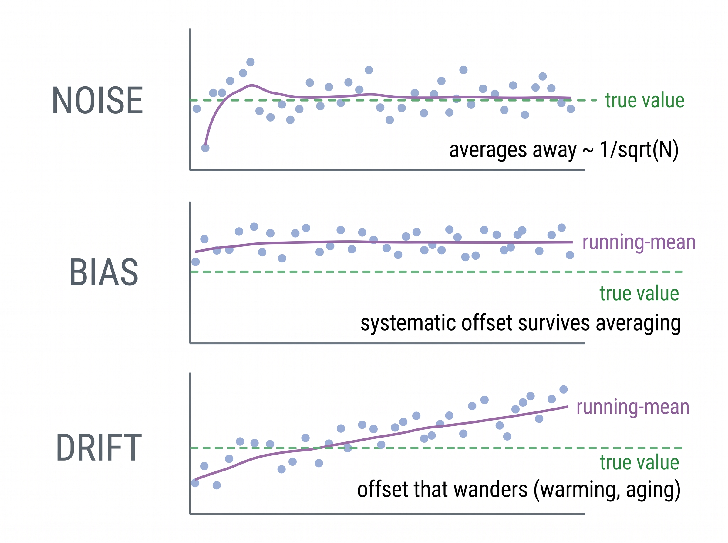
Case B, add a \(+0.5\) bias. Every reading shifts up by \(0.5\), giving \(21.8,\ 19.4,\ 21.1,\ 20.1\). The running means become \(21.8,\ 20.6,\ 20.77,\ 20.60\), and no matter how many more readings you add they converge on \(20.5\), never \(20.0\). The noise still averages away exactly as before, but the \(0.5\) offset sits in every term of the sum, so it survives the division untouched. That is the whole lesson of this section in nine numbers: more data cures randomness and is powerless against a systematic error.
Bias is a systematic offset: the reading is consistently wrong in the same direction. A cheap accelerometer at rest rarely reports zero; it reports a small, stubborn nonzero vector. Averaging makes bias more visible, not less, because it does not cancel.
Drift is bias that will not hold still. As a component warms up, ages, or its supply voltage sags, its zero point wanders. The calibration you performed this morning is typically already slightly stale by afternoon. Drift is why "calibrate once and forget" is a fantasy and why Chapter 9 spends real effort tracking a slowly-moving bias as part of the hidden state rather than pretending it is constant. Figure 1.1.1 illustrates noise vs. bias vs. drift, and what averaging can and cannot fix.
Key Insight
Noise, bias, and drift are not correctable accidents you engineer away; they are the signature of measurement itself. The professional move is not to eliminate them but to model them: to write down how large the noise is, which direction the bias leans, and how fast the drift creeps, and then to reason under that uncertainty. A sensor with well-characterized error is worth more than a "better" sensor whose error you do not understand.
Two quick vignettes make the point physical. Leave a thermometer in direct sunlight and it will happily report the temperature of a sunbaked plastic case, not the air; the instrument faithfully measured the wrong thing, and its reading is a confident lie. Set a smartphone flat on a table and its accelerometer reports roughly \(9.8\ \mathrm{m/s^2}\) pointing up, because an accelerometer cannot separate the specific force, which is the acceleration a sensor feels relative to free fall, of gravity from genuine motion. It is not broken. It is telling you the literal truth about force, which is not the question you asked. In both cases the number is real and the interpretation is a trap.
Common Misconception
The misconception is that a sensor which reports the "wrong" answer must be malfunctioning, so a better or more expensive unit would fix it. The sunlit thermometer and the resting accelerometer are working flawlessly and reporting exact physical truth; the error lives in your interpretation of the number, not in the hardware, which is why a pricier sensor buys you nothing here and honest modeling of what the instrument actually measures buys you everything.
Perception is an inverse problem
Put the pieces together and a shape emerges. Physics runs forward: a hidden state \(s\) causes a signal through some sensor response \(h(\cdot)\), corrupted by measurement noise \(\eta\). Written compactly, and stripped of every subtlety that Chapter 2 will restore,
\[ x = h(s) + \eta. \]You never get \(s\). You get \(x\), and your job is to run the arrow backward: recover the cause \(\hat{s}\) from the effect \(x\). This is an inverse problem, hard for a specific reason. Because \(h(\cdot)\) is many-to-one and \(\eta\) is random, many states \(s\) fit the same \(x\), so inversion is never pure deduction; it is inference under uncertainty. The right output is not one confident answer but a distribution over states, the posterior \(p(s \mid x)\) that Chapter 4 builds from the ground up.
Mental Model
Think of a shadow puppet on a wall. A three-dimensional hand, held in front of a lamp, casts a flat outline; going from hand to shadow is the forward direction, quick and determined by simple geometry. Now try the reverse: shown only the shadow, name the exact hand pose that made it. You cannot, because the wall records outline but discards depth, so a rabbit, a bird, and countless slightly different finger arrangements all cast the same shape. That is the inverse problem exactly: the sensor is the lamp-and-wall projection that throws away dimensions, and recovering the state from the signal is guessing the hand from its shadow, so the honest answer is a set of plausible poses, not one.
The diagram in Figure 1.1 traces this loop. The world holds a rich hidden state; the sensor squeezes it through \(h(\cdot)\) and adds \(\eta\), yielding a thin signal \(x\); and inference reaches back across that lossy channel to propose \(\hat{s}\), always with a margin of doubt attached.
Figure 1.1. Physics runs the arrow forward, from hidden state \(s\) through the sensor response \(h(\cdot)\) and added noise \(\eta\) to a signal \(x\). Perception runs it backward, recovering an estimate \(\hat{s}\) that must carry a margin of doubt.
Research Frontier
The inverse problem \(p(s \mid x)\) that this section sketches by hand is now being solved with learned priors. "Diffusion Posterior Sampling for General Noisy Inverse Problems" (Chung et al., ICLR 2023) uses a diffusion model as a rich prior over plausible states and draws samples from the posterior for a broad family of corruptions, blur, missing data, and nonlinear noise, without retraining for each new task. Where Section 1.1 writes the error model by hand and returns a single estimate, methods in this line learn the prior from data and return a whole distribution of candidate states, turning "attach a margin of doubt" from a slogan into calibrated samples you can actually compute.
In Practice
A wrist wearable estimates heart rate with photoplethysmography (PPG): a green light-emitting diode (LED) shines into the skin and a photodiode measures how much light the pulsing blood absorbs. On a still wrist the signal is a clean periodic wave and the rate is easy. Start running, and the same photodiode now sees light modulated by tendons sliding, the band bouncing, and ambient sunlight leaking in at exactly the cadence of your stride. The device can lock onto your step rate and report it as your heart rate with total confidence. This is the inverse problem failing in the field: two very different states, "heart beating at 150" and "arm swinging at 150," produce nearly identical light. The fix is not a purer sensor. It is fusing PPG with the accelerometer to explain away the motion, a strategy this book develops fully in Chapter 30.
No single sensor gives you ground truth
Here is the conclusion that reorganizes everything. Because measurement is a lossy, biased, drifting projection, and because inversion is ambiguous, a single reading is a claim, not a fact. The thermometer claims the air is warm; the PPG sensor claims the heart beats at 150; the accelerometer claims a force. Each claim is evidence, weighted by how much you trust the instrument that made it, and evidence can be wrong. Treating one sensor's output as ground truth is the original sin of applied sensing. In practice, a great many field failures trace back to it: a drone that flips because it trusted a single bad gyro reading, a monitor that pages a nurse over a motion artifact.
This is precisely why the rest of the book exists. If one sensor cannot be trusted, you characterize its error (calibration), you suppress what you can and quantify what remains (filtering and uncertainty), you combine independent instruments so their errors cancel rather than compound (fusion), and you keep tracking the drift while the system runs (state estimation). Every one of those chapters is a different answer to the same sentence: the instrument mediates everything, so knowing the instrument is the prerequisite to trusting the data.
Real-World Application: commercial aviation
Boeing's 737 MAX Maneuvering Characteristics Augmentation System (MCAS) flight-control system read the aircraft's angle of attack, which is the angle between the wing and the oncoming airflow, from a single vane sensor and, when that one vane jammed with a false high reading, repeatedly pushed the nose down against the pilots, a chain that ended in two crashes. The redesign did exactly what this section prescribes: MCAS now compares two independent angle-of-attack sensors and disables itself when they disagree, treating each reading as a contestable claim rather than ground truth. A modern airliner already carries triple-redundant air-data and inertial units for the same reason, so a single instrument can never silently steer the decision.
The Right Tool
Suppose you want to strip a slow drift out of a signal before analysis. Written from first principles you would fit a trend line by least squares (the standard best-fit criterion), evaluate it at every sample, and subtract, roughly a dozen lines of index-juggling that are easy to get subtly wrong at the window edges. A mature library collapses that to one call:
from scipy.signal import detrend
x_clean = detrend(x) # removes a fitted linear drift from xscipy.signal.detrend(x) call fits a linear trend by least squares, evaluates it at every sample, and subtracts it, collapsing roughly a dozen lines of edge-sensitive index-juggling into one. It does not decide whether removing that drift is correct; that judgment is yours.As Listing 1.1 shows, the library removes the drudgery, not the responsibility. Deciding that a linear detrend is the right model, rather than a symptom you should have tracked as state, remains a modeling choice this book keeps returning to.
Aside
An accelerometer at rest insisting it feels \(9.8\ \mathrm{m/s^2}\) is not lying. It has simply never heard of the ground and cannot tell "being pushed up by a table" from "accelerating skyward through empty space." Einstein built a theory of gravity on that exact confusion. Your step counter inherits it for free, and mostly just miscounts stairs.
Exercise
Pick a sensor you own: a phone accelerometer, a smartwatch heart-rate monitor, or a kitchen meat thermometer. Write down three distinct physical situations in which it would report a reading that is technically correct yet answers a different question than the one you meant to ask. For at least one of them, name a second, cheap sensor whose reading would let you detect that the first was misleading. Keep this list; you are sketching your first sensor-fusion design.
Self-Check
1. Why can averaging many readings reduce noise but not bias?
2. In \(x = h(s) + \eta\), which term makes recovering \(s\) an inverse problem rather than a lookup, and why?
3. Restate "a single reading is a claim, not a fact" in terms of partial observability. Why does many-to-one projection forbid single-sensor ground truth?
Try It: Watch bias survive averaging
In about twenty lines of NumPy you can see with your own eyes that averaging defeats noise but is helpless against bias and drift, the central claim of this section.
- Simulate a true constant value of \(20.0\) with added noise:
import numpy as np; N = 10000; readings = 20.0 + 0.5 + np.random.normal(0, 2.0, N). The0.5is a fixed bias, the normal draw is the noise. - Compute the running mean over the first \(k\) samples with
running = np.cumsum(readings) / np.arange(1, N + 1)and plot it withmatplotlib.pyplot. Watch it settle onto \(20.5\), not \(20.0\): the noise averages away, the \(0.5\) bias does not. - Add a slow drift: rebuild the signal as
readings = 20.0 + 0.5 + 0.001 * np.arange(N) + np.random.normal(0, 2.0, N), recompute the running mean, and confirm it now chases a moving target instead of converging at all. - Pass the drifting signal through
from scipy.signal import detrend; cleaned = detrend(readings), plot its running mean, and verify the linear drift is gone while the constant offset issue you introduced in step 1 is a separate problem detrend never touches.
The one-line takeaway you can now demonstrate: more data cures randomness, never a systematic error.
Lab: feel your phone's accelerometer bias and drift
Goal. Confirm empirically that a real inertial sensor at complete rest reports a nonzero, temperature-dependent bias that averaging cannot remove, the exact claim this section makes about bias and drift.
Tools. Any smartphone with the free phyphox app (or an Arduino/Raspberry Pi with an MPU-6050 inertial measurement unit (IMU)), plus Python with NumPy and Matplotlib. Budget 15 to 30 minutes.
Procedure. Lay the phone flat and motionless on a table. In phyphox open "Acceleration (without g)," record for 60 seconds, and export the comma-separated values (CSV) file. The true specific force along every axis is now zero, so anything nonzero you see is bias plus noise. Load it in Python and compute the per-axis mean and standard deviation:
import numpy as np
a = np.loadtxt("accel.csv", delimiter=",", skiprows=1)  # t, ax, ay, az
print("mean (bias):", a[:, 1:].mean(axis=0))
print("std (noise):", a[:, 1:].std(axis=0))mean of the three acceleration columns is the sensor's bias (it should be zero at rest but is not), while the per-axis std is the noise you can average down. The two lines separate the offset that survives averaging from the jitter that does not.What to vary. (1) Record again after warming the phone in your hands or cooling it briefly in a fridge bag, and compare the means: the bias shifts with temperature, which is drift. (2) Change the averaging window by taking the running mean over the first \(k\) samples and watch the noise shrink like \(1/\sqrt{k}\) while the bias flatlines at a nonzero value.
What to observe. The mean never lands on zero, the running mean converges to that same nonzero bias rather than to zero, and the bias you measured cold differs from the one you measured warm. You have just reproduced, on hardware in your pocket, why "calibrate once and forget" fails and why Chapter 9 tracks bias as part of the state.
What's Next
Section 1.2 turns the smudged-pane idea into a working distinction: why building AI on physical measurements differs so sharply from building AI on text and pixels, and why the presence of an instrument between the model and the world changes almost every design decision that follows.